Super Chill Guide to Simple Linear Regression in R 2024

Hey There, Future Data Wiz! 🌟
What’s Simple Linear Regression and Why Should You Care? 🤔
Hey fam! 🙌 So you’re here to become a data wizard, right? Well, you’re in the perfect spot! Let’s kick things off with something called Simple Linear Regression. Sounds fancy, huh? Don’t worry; it’s simpler than it sounds. 🤓
Imagine you’re trying to predict how many likes your next TikTok video will get based on the number of hours you spent making it. You’ve got some data from your past videos, and you want to make an educated guess for the future. That’s where Simple Linear Regression comes in! 🎥💫
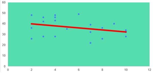
In the simplest terms, Simple Linear Regression is like drawing a straight line through a bunch of data points to predict future values. It’s like connecting the dots but in a super smart way! 📈
Contact for free consultation and lectures
Why Simple Linear Regression is the Go-To Tool for Data Newbies and Pros Alike! 🛠️
Okay, so you get that Simple Linear Regression is cool for predicting stuff. But guess what? It’s not just for TikTok likes! This tool is super versatile and can be used in so many areas. 🌍
- Gaming Stats: Wanna know how your performance in a game might improve over time? Simple Linear Regression can help you level up! 🎮
- Social Media Trends: Curious about how trends grow and fade on platforms like Twitter or Instagram? Yep, you guessed it—Simple Linear Regression to the rescue! 📸
- School Grades: Want to predict your final grade based on your current performance? This tool has got your back! 📚
- Fitness Goals: Trying to figure out how much weight you’ll lose by sticking to your new diet? Simple Linear Regression can give you a sneak peek into your fit future! 🏋️♀️
- Stock Market: If you’re into investing, this tool can help you make some educated guesses about stock prices. Just remember, the stock market is a bit more complicated, so use it wisely! 💰
So, are you pumped to dive into the world of Simple Linear Regression? Trust me; by the end of this guide, you’ll be a pro at predicting all sorts of things! 🚀 Let’s get started! 🌈💖
What is the the formula of Simple Linear Regression? The ABCs 📚
The Magic Formula That Makes It All Happen 🪄
Alright, fam, let’s get into the nitty-gritty! 🤩 Simple Linear Regression has a magic formula that makes everything click. The formula looks like this:
Y = a + bX
Hold up, don’t freak out! 🙅♀️ Let’s break it down:
- Y: This is what you’re trying to predict. It could be your future TikTok likes, your final grade in a class, or even the price of a stock. 🎯
- a: This is the starting point of your line on the graph. Think of it as the base number of likes you’ll get on TikTok, even if you just post a black screen. 🖤
- b: This is the slope of the line. It shows how much your “Y” (like TikTok likes) will change when your “X” changes. 📈
- X: This is your input or what you’re using to make the prediction. It could be the number of hours you spent making a video, the number of classes you’ve attended, etc. ⏳
Terminologies of Simple Linear Regression – The Lingo You Gotta Know 🗣️
Okay, so you’ve met the stars of the show (the formula elements), but there’s some backstage lingo you gotta know to truly get Simple Linear Regression. 🎤
- Dependent Variable: This is another name for “Y.” It’s what you’re trying to predict. 🎯
- Independent Variable: This is your “X.” It’s what you’re using to make the prediction. 🎲
- Coefficient: This is a fancy term for the “b” in the formula. It tells you the relationship between X and Y. 💑
- Intercept: This is the “a” in the formula. It’s where your line starts on the graph. 🏁
- Residuals: These are the differences between the actual data points and the points on the line. Think of them as the “oopsies” in your predictions. 😬
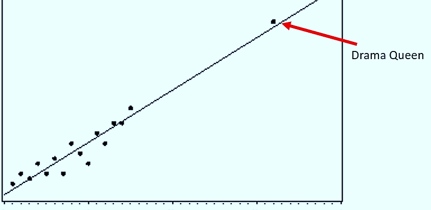
- Outliers: These are the drama queens—data points that don’t really fit with the rest. 👑
- Fit: This is how well your line matches the data points. A good fit = a happy model. 😃
So, how are we feeling? Ready to become a Simple Linear Regression superstar? 🌟 Let’s keep the good vibes rolling! 🌈💖
Conditions of Simple Linear Regression – The Rulebook 📜
Assumptions of Simple Linear Regression –
The Do’s and Don’ts You Need to Know 🤓
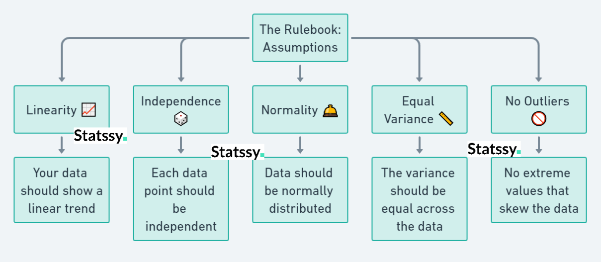
Hey there, future data guru! 🌟 Before we jump into the fun stuff, we’ve got to talk about some ground rules. Every game has its rulebook, right? 🎮 Well, Simple Linear Regression is no different. Understanding these rules or ‘assumptions’ is super important because if we ignore them, our predictions could be way off! 😱 So, let’s get into it.
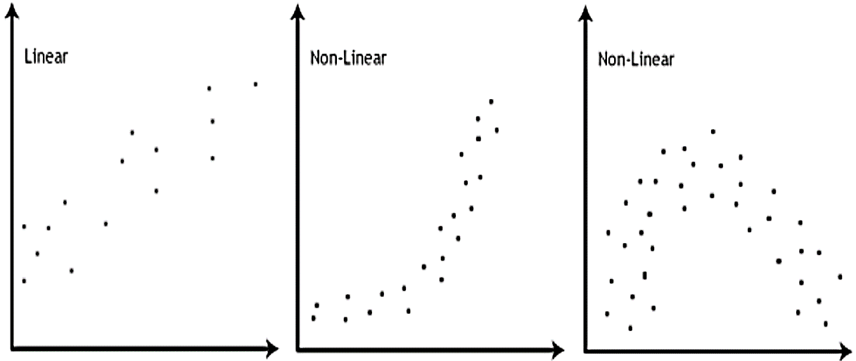
1. Linearity Assumption 📈
First up is Linearity. This one’s all about making sure your data fits a straight line. Imagine you’re drawing a line through your TikTok likes based on how many hours you spent on each video. If the likes and hours don’t follow a straight line, then Simple Linear Regression might not be the best tool for you. Think of it like trying to fit a square peg into a round hole—it just won’t work! 🚫
2. Independence Assumption 🎲
Next, we have Independence. This means that each piece of data you collect should not depend on any other data point. So, if you’re using Simple Linear Regression to predict your grades, each test score should be its own unique thing, not influenced by your other test scores. It’s like rolling a dice; each roll is independent of the last one. 🎲
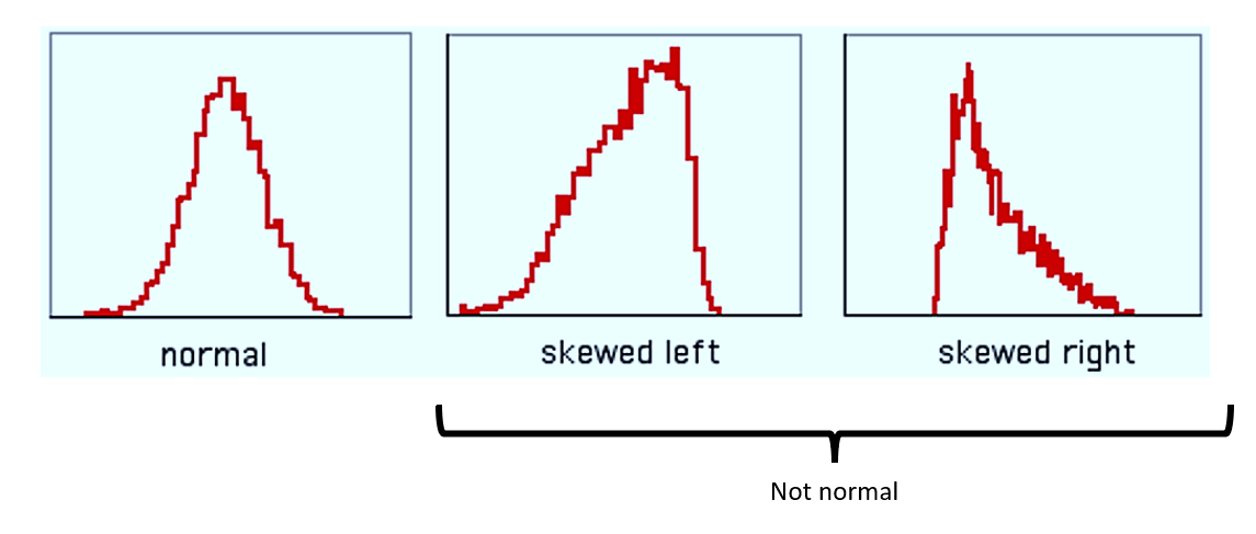
3. Normality Assumption 🛎️
Normality is all about the shape of your data. When you plot all your data points, they should form what’s called a ‘normal distribution,’ which looks like a bell. 🛎️ This is super important because if your data is skewed to one side, your predictions could be off. So, make sure your data is as bell-shaped as possible!
4. Equal Variance Assumption – Heterosckedasticity 📏
Equal Variance is a fancy way of saying that the spread of your data should be even. Imagine you’re throwing darts at a dartboard. If all your darts land in different corners, that’s not equal variance. You want your darts—or in our case, data points—to be evenly spread out. 🎯
5. No Outliers 🚫
Last but not least, watch out for outliers. These are the drama queens of the data world. 👑 They’re extreme values that don’t fit with the rest of your data. Outliers can seriously mess up your predictions, so it’s best to identify and deal with them early on.
So there you have it! Those are the key assumptions or ‘rules’ you need to keep in mind when working with Simple Linear Regression. Trust me, understanding these will make your data journey so much smoother. 🛣️
Let me give you a flowchart
Advantages and Disadvantages of Simple Linear Regression – The Good, the Bad, and the Ugly 😇😐😬
The Perks 🎉
Why Simple Linear Regression Rocks! 🤘
Simple Linear Regression is like that reliable friend who’s always there when you need them. Let’s talk about why it’s so awesome:
- Easy to Understand 🧠: One of the best things about Simple Linear Regression is that it’s super easy to grasp. You don’t need a PhD in Math to get it. It’s like understanding the rules of a basic video game; you catch on pretty quickly!Example: Imagine you want to predict your final grade in a course based on the number of hours you study. Simple Linear Regression can help you do that in a way that’s easy to understand. More study hours = better grades, right? 📚
- Quick to Use ⏱️: You can get results fast, which is perfect for when you’re in a hurry to prove a point or make a decision.Example: Let’s say you’re a streamer and you want to know how many views you’ll get if you stream for 5 hours a day. Simple Linear Regression can give you a quick answer! 🎮
- Versatile 🛠️: You can use it in various fields like marketing, finance, healthcare, and even in your daily life.Example: From predicting stock prices 📈 to figuring out how effective a new diet plan will be 🥗, this tool has got you covered.
- Low Cost 💵: You don’t need fancy software or powerful computers. Even a basic laptop can run Simple Linear Regression models.Example: You can run a Simple Linear Regression model on your 5-year-old laptop and still get reliable results. No need for a supercomputer! 🖥️
Example: You can run a Simple Linear Regression model on your 5-year-old laptop and still get reliable results. No need for a supercomputer! 🖥️
The Downsides 😕
Where Simple Linear Regression Kinda Falls Short 🤷♀️

Now, no one’s perfect, right? Simple Linear Regression has its limitations too:
- Overly Simplistic 🌈: It only considers one independent variable, which might not capture the complexity of real-world situations.
Example: If you’re trying to predict your final grade, just looking at study hours might not be enough. What about attendance, participation, or previous knowledge? 🤔
- Sensitive to Outliers 👀: A single outlier can skew your entire model, leading to inaccurate predictions.
Example: Imagine you’re predicting the price of a sneaker based on its brand. If one pair is diamond-encrusted and costs $10,000, it could throw off your whole model. 💎
- Assumptions Galore 📜: As we discussed earlier, there are several assumptions you have to meet, which can be a bit of a hassle.
Example: If your data doesn’t fit a straight line or if the data points are not independent, you’ll have to either transform your data or choose a different model. 🔄
- Limited Predictive Power 🔮: It’s great for understanding relationships between two variables, but it’s not the best for making future predictions.
Example: You might be able to predict tomorrow’s weather based on today’s, but don’t count on it for a long-term forecast. 🌦️
So, that’s the good, the bad, and the ugly of Simple Linear Regression. Knowing both sides of the coin will help you use this tool more effectively. 🌟 🚀
|
Aspect |
Description |
Example |
|
|
Perks 🎉 |
|||
|
Easy to Understand 🧠 |
Simple to grasp, no advanced math needed. |
Predicting grades based on study hours. |
🧠 |
|
Quick to Use ⏱️ |
Get results fast, perfect for quick decisions. |
Predicting stream views based on hours streamed. |
⏱️ |
|
Versatile 🛠️ |
Applicable in various fields like marketing, finance, etc. |
Predicting stock prices or diet plan effectiveness. |
🛠️ |
|
Low Cost 💵 |
No need for fancy software or powerful computers. |
Can run on a basic laptop. |
💵 |
|
Downsides 😕 |
|||
|
Overly Simplistic 🌈 |
Considers only one independent variable. |
Predicting grades might need more than just study hours. |
🌈 |
|
Sensitive to Outliers 👀 |
A single outlier can skew the model. |
A diamond-encrusted sneaker can throw off price predictions. |
👀 |
|
Assumptions Galore 📜 |
Must meet several assumptions for accurate results. |
Data must fit a straight line and points must be independent. |
📜 |
|
Limited Predictive Power 🔮 |
Not the best for making long-term predictions. |
Good for predicting tomorrow’s weather, not long-term. |
🔮 |
This table format makes it easy to compare the good and the not-so-good aspects of Simple Linear Regression. It’s a quick reference guide for you into this topic! 🌟
Let’s Get Coding in R! 🤖
Alright, enough chit-chat. Let’s get our hands dirty with some coding! 🎉 Don’t worry if you’ve never coded before; I’ll walk you through it step-by-step. 🤗
Setting Up R Studio – Your Playground 🌈
Before we dive into the code, we need to set up our R environment. Think of it as setting up your gaming console before playing. 🎮
- Install R: If you haven’t already, download and install R from here.
- Install RStudio: This is where the magic happens. It’s like the dashboard of your car but for R. Download it from here.
# Hey there! 👋 Let's install a package!
install.packages("ggplot2") # This package is for cool graphs 📊
Your First Simple Linear Regression Code: Let’s Predict Your TikTok Followers! 🕺💃
Okay, now that we’re all set up, let’s write our first Simple Linear Regression code. We’re going to predict how many TikTok followers you’ll have based on the number of videos you post. 📹
- Load the Data: First, we need some data to work with. Let’s say you’ve kept track of your TikTok followers and the number of videos you’ve posted.
- Run the Model: We’ll use the lm()function in R to create our model. lm stands for ‘linear model,’ by the way. 🤓
# Let's get this party started! 🎉
# Your Instagram data for an entire month 📅📹
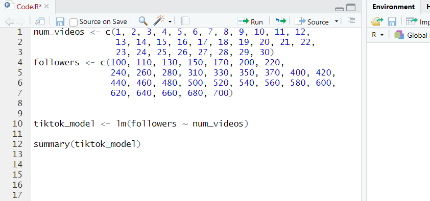
num_videos <- c(1, 2, 3, 4, 5, 6, 7, 8, 9, 10, 11, 12, 13, 14, 15, 16, 17, 18, 19, 20, 21, 22, 23, 24, 25, 26, 27, 28, 29, 30)  # Number of videos you've posted in 30 days
followers <- c(100, 110, 130, 150, 170, 200, 220, 240, 260, 280, 310, 330, 350, 370, 400, 420, 440, 460, 480, 500, 520, 540, 560, 580, 600, 620, 640, 660, 680, 700)  # Your followers in 30 days
# Time to run our model 🚀
tiktok_model <- lm(followers ~ num_videos)  # 'followers' is what we're predicting, 'num_videos' is what we're using to predict!
# Let's see how we did 🤩
summary(tiktok_model)  # This will show us all the juicy details!
If you copy page this code in R Studio, you will something like this
Try running the code using “Run” button. When you do that you will get something like this. We will understand everything what it generates.
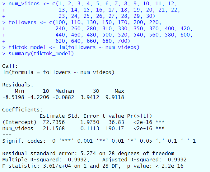
And there you have it! You've just run your first Simple Linear Regression model in R! 🌟 How does it feel to be a coding wizard? 🧙♂️ Ready for the next adventure? 🚀
lm Function in R : Your New BFF in R 👯♀️
So, you've got your R environment set up, and you've even run your first Simple Linear Regression model. High five! 🙌 But wait, you're probably wondering what that lm() thing was all about, right? Well, let me introduce you to lm(), your new Best Friend Forever in the world of R! 🎉
What's lm() and Why It's Awesome 🌈
The lm() function is like the Swiss Army knife of linear models in R. It's short for "Linear Model," and it's the go-to function for running Simple Linear Regression. But that's not all; it can handle multiple linear regression, polynomial regression, and more! 🤯
Here's why lm() is so cool:
- User-Friendly 🤗: You don't need to be a coding genius to use lm(). It's super straightforward. You tell it what you want to predict and what you're using to make that prediction, and voila! 🎩✨
- Informative 📚: Once you run lm(), you can use the summary()function to get all the nitty-gritty details about your model. It's like getting the behind-the-scenes tour of a movie set. 🎬
- Flexible 🤸♀️: You can use lm()for more than just Simple Linear Regression. As you get more comfortable with it, you'll find it's versatile enough for more complex models too. 🛠️
- Community Support 🤝: Because lm()is so popular, there's a ton of tutorials, forums, and online help available. It's like having a 24/7 tech support team! 🌐
Here's a code snippet to show you how easy it is to use lm():
# Let's use lm() to predict TikTok followers based on the number of videos 🤩
my_model <- lm(followers ~ num_videos)  # 'followers' is our dependent variable, 'num_videos' is our independent variable

So, are you ready to make lm() your new BFF in R? Trust me, once you get to know it, you'll wonder how you ever lived without it! 🌟 Let's keep going! 🚀
Interpreting Simple Linear Regression 🚀
Now let’s interpret what we got. Don’t worry if it looks scary, we will break down everything.
1) The Coefficients of SLR : The Secret Sauce 🍯
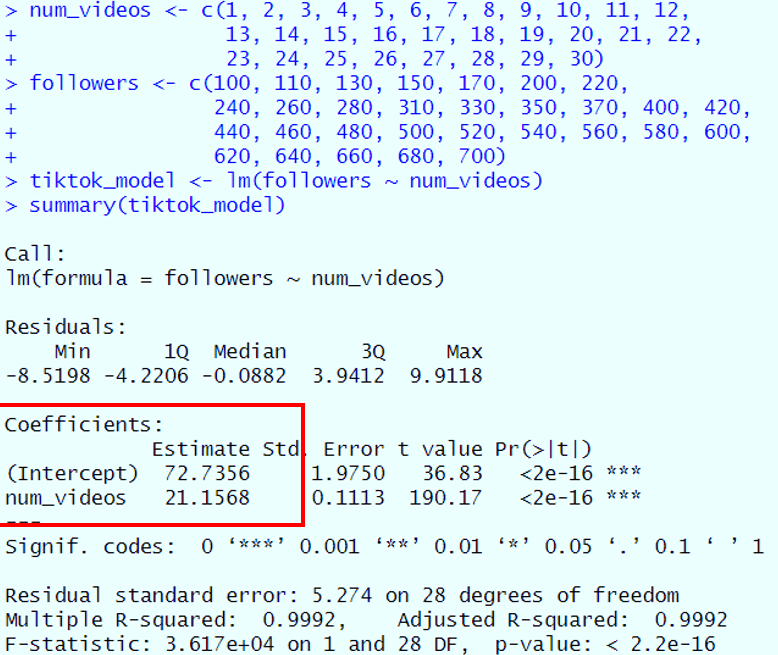
Alright, let's dig into the heart of your TikTok model—the coefficients! These are the magical numbers that help us understand how the number of videos you post is related to your follower count. 🌟
The Intercept 🛑
What it is:
The intercept is like your starting line in a race. Imagine you're at a TikTok marathon, and even before you start running (or in this case, posting videos), you already have some followers cheering you on. That's what the intercept is! In our model, the intercept is 72.7356.
What it means:
This number tells us that even if you haven't posted a single video, you'd still have around 73 followers. Maybe they're friends, family, or people who just love your profile pic! 🤷♀️
How to interpret it:
The intercept is super important because it sets the baseline for your model. If the intercept is high, it means you're starting off strong. If it's low, don't worry—you can make it up by posting awesome videos! 🎥
The Slope 📈
What it is:
The slope is like your pace in the TikTok marathon. It tells you how fast you're gaining followers as you keep posting videos. In our model, the slope is 21.1568.
What it means:
For every video you post, you can expect to gain around 21 new followers. That's like adding a small classroom of fans for every video! 🎉
How to interpret it:
A high slope means each video has a big impact, while a low slope means you'll need to post more videos to see a significant increase in followers. Either way, the slope helps you strategize your TikTok game. 🌟
Summary Table 📊
|
Term |
Value |
What it Means |
How to Interpret it |
|
Intercept 🛑 |
72.7356 |
The number of followers you'd have even if you posted zero videos. |
A high number means you're starting off strong. |
|
Slope 📈 |
21.1568 |
The number of new followers you gain for each additional video you post. |
A high number means each video has a big impact. |
Mathematically you can write it as,


2) The Goodness: R-squared and Adjusted R-squared 🌟
Before going into these complexities let us do a primary check also
The Connection: Correlation 101 🤝
First up, let's talk about correlation. This is basically your relationship status with your data. Are you just friends, or is it a match made in heaven? 😍
What's Correlation and Why It's Your Relationship Status with Data 💕
- Positive Correlation: When one variable goes up, the other goes up too. It's like you and your BFF always showing up in matching outfits. 👯♀️
- Negative Correlation: When one variable goes up, the other goes down. Think of it like a see-saw. 🙃
- No Correlation: No relationship at all. Like, you don't even know her. 🤷♀️
Here's a code snippet to find the correlation:
# Let's find out our relationship status 🤝
cor(num_videos, followers)
When you run this code, you will get this value of correlation.

So how do we interpret it?
|
Correlation Coefficient Range |
Strength |
Relationship Status |
Suitable for Regression? |
|
-1 to -0.5 |
Strong |
Like oil and water 🛢️💧 |
Yes, strongly advised |
|
-0.5 to 0 |
Weak |
Casual acquaintances 🙋♀️👋 |
Proceed with caution |
|
0 |
None |
Don't know her 🤷♀️ |
Not advised |
|
0 to 0.5 |
Weak |
Just friends 👫 |
Proceed with caution |
|
0.5 to 1 |
Strong |
BFFs forever 👯♀️ |
Yes, strongly advised |
- Strong: A strong correlation means the variables are closely related and move almost in sync. It's like they're finishing each other's sentences. 🥺
- Weak: A weak correlation means the variables kinda know each other but aren't really hanging out. It's like that friend you only see at parties. 🎉
- None: No correlation means these variables are basically strangers. They don't interact, and they don't influence each other. 🚶♀️🚶♂️
- Suitable for Regression?: This column tells you if linear regression is a good technique to model the relationship between these variables. If it's "strongly advised," go for it! If it says "proceed with caution," you might want to consider other factors or techniques. 🤓
So here we have 0.9996131 which means BFFs forever.
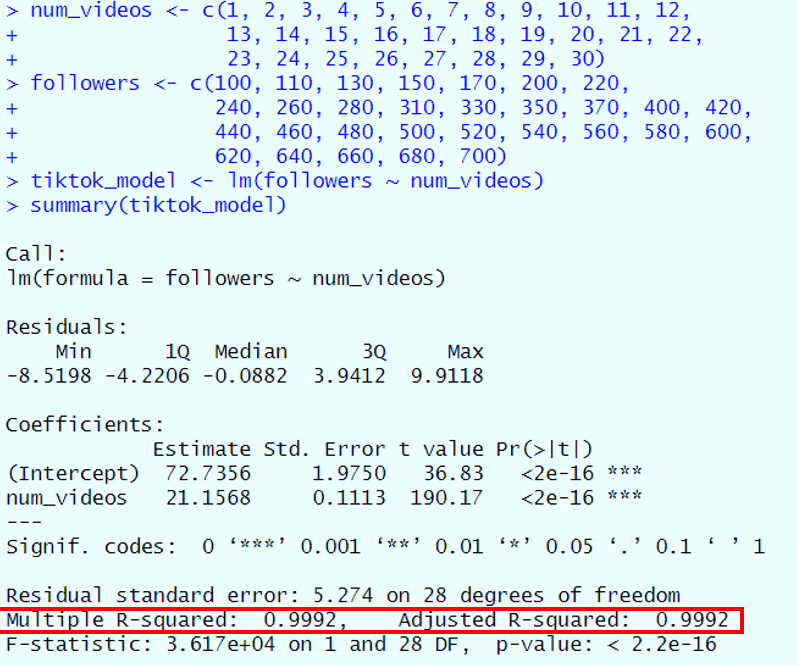
So, you've run your TikTok model and you're probably wondering, "Is my model any good?" 🤔 Enter R-squared and Adjusted R-squared—your model's report card!
R-squared 📏
What it is:
Think of R-squared as your model's grade in school. It's a number between 0 and 1 that tells you how well your model fits the data. The closer to 1, the better the fit!
What it means:
In our TikTok example, the R-squared value is 0.9992, which is super close to 1. This means your model is like the valedictorian of TikTok predictions! 🎓
How to interpret it:
- 0 to 0.3: Your model needs some extra tutoring. 📚
- 0.4 to 0.6: Not bad, but there's room for improvement. 🆗
- 0.7 to 0.9: You're on the honor roll! 🏆
- 0.9 to 1: You're the TikTok prediction genius! 🌟
Adjusted R-squared 📐
What it is:
This is like R-squared's sophisticated cousin. It adjusts the R-squared value based on the number of predictors in your model. It's a bit more cautious and can penalize your model for adding unnecessary variables.
What it means:
In our example, the Adjusted R-squared is also 0.9992, which means not only does your model fit the data well, but it's also not overly complicated. 🌟
How to interpret it:
Adjusted R-squared helps you keep it real. If you add too many unnecessary variables, this number will drop, telling you to simplify your model.
Summary Table 📊
|
Term |
Value |
What it Means |
How to Interpret it |
|
R-squared 📏 |
0.9992 |
The proportion of the variance in the dependent variable that is predictable from the independent variable(s). |
Closer to 1 means better fit. |
|
Adjusted R-squared 📐 |
0.9992 |
The proportion of the variance in the dependent variable that is predictable, adjusted for the number of predictors. |
Closer to 1 means better fit without unnecessary complexity. |
This mind map and table should give you a comprehensive understanding of R-squared and Adjusted R-squared. So, how did your model score? 🌟

3) The Judge: F-statistic and p-value ⚖️
Alright, let's get into the courtroom drama of data science! The F-statistic and p-value are like the judge and jury of your model. They tell you if your model is statistically significant or not. 🕵️♀️
F-statistic 📊
What it is:
The F-statistic is like the judge's gavel. It's a number that helps you understand if your model is significant or just random noise.
What it means:
In our TikTok example, the F-statistic is 3.617e+04. That's a big number, and in the world of statistics, bigger is usually better. It means that the relationship between the number of videos and followers is not just by chance.
How to interpret it:
- Small F-statistic: Uh-oh, your model might not be significant. 🤨
- Large F-statistic: Yay, your model is likely significant! 🎉
p-value 🅿️
What it is:
The p-value is like the jury's verdict. It tells you the probability that your results are due to random chance.
What it means:
In our example, the p-value is < 2.2e-16, which is basically zero. This means there's almost no chance that the relationship we're seeing is random.
How to interpret it:
- p-value > 0.05: Your model is not significant. 😕
- p-value <= 0.05: Your model is significant. 🌟
Summary Table 📊
|
Term |
Value |
What it Means |
How to Interpret it |
|
F-statistic 📊 |
3.617e+04 |
Measures how well the model fits compared to a model with no predictors. |
Larger value means the model is likely significant. |
|
p-value 🅿️ |
< 2.2e-16 |
The probability that the observed relationship happened by chance. |
Smaller value (usually <= 0.05) means the model is significant. |
So, is your model ready for the red carpet or does it need a makeover? 🤔

Make It Pretty: Data Viz Time 🎨
Okay, so you've got your data and your model, but let's be real—numbers on a screen can be a snooze-fest. 😴 Time to jazz things up with some data visualization! 🎨 Trust me, it's not just for the 'gram; it actually helps you understand your data better. 🌈
Scatter Plots with ggplot2: Because Dots are Cute 🌈
First up, let's talk scatter plots. These little guys are basically a bunch of dots on a graph that show you how two variables interact. And guess what? We're going to make them using ggplot2, the Beyoncé of R packages. 🌟
How to Make Your Data Points Look Fab 💅
- Install ggplot2: If you haven't already, you'll need to install the ggplot2 package. It's like downloading a new app for your phone.
- Plot It: Use the ggplot()function to create your scatter plot.
Here's a code snippet to get you started:
# First, let's install ggplot2 📦
install.packages("ggplot2")

# Now, let's make a scatter plot 🌈
library(ggplot2)  # Load the package
ggplot(data = data.frame(num_videos, followers), aes(x = num_videos, y = followers)) +
geom_point(aes(color = followers), size = 4) +  # Make the points colorful and cute!
theme_minimal()  # Minimalist theme for that clean look
And voila! You'll get a colorful scatter plot that's as cute as a button. 🌈
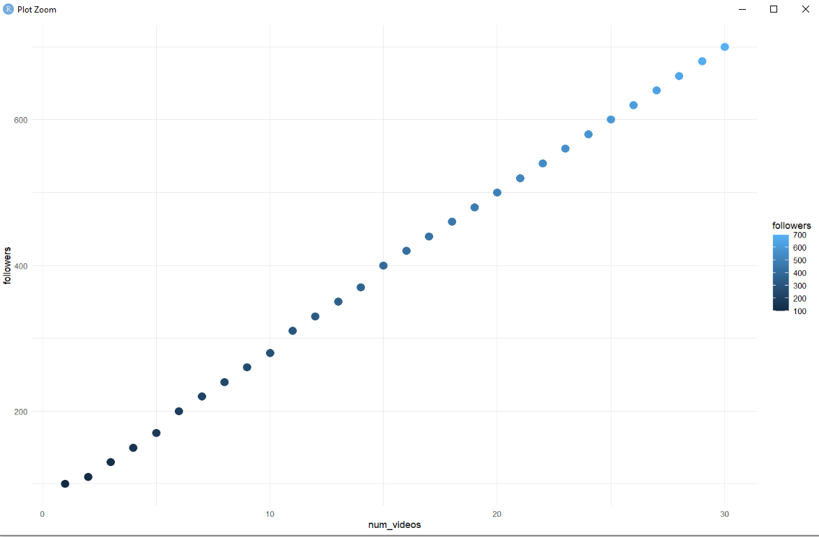
The Line of Best Fit: Your Trendsetter 👠
Now, let's add a line of best fit to our scatter plot. This line helps us see the general trend of our data. It's like the fashion trendsetter of the data world. 👠
How to Draw That Perfect Line 💁♀️
- Add the Line: Use the geom_smooth()function to add a line of best fit to your scatter plot.
- Glam It Up: You can customize the line's color, type, and more!
Here's another code snippet for you:
# Let's add a line of best fit 👠
ggplot(data = data.frame(num_videos, followers), aes(x = num_videos, y = followers)) +
  geom_point(aes(color = followers), size = 4) +  # Our cute points
  geom_smooth(method = "lm", se = FALSE, color = "pink") +  # The line of best fit in fabulous pink
  theme_minimal()  # Keep it clean
And there you have it—a glam-up scatter plot complete with a line of best fit! 🌟
So you can clearly see that actual data points are a bit deviating from the main line but still we are able to approximately touch many of the points. It is because the regression aims to touch as many points as possible.
So, are you ready to make your data look runway-ready? 🎉 Let's strut our stuff into the next section! 🚀
Residuals: The Leftover Tea ☕
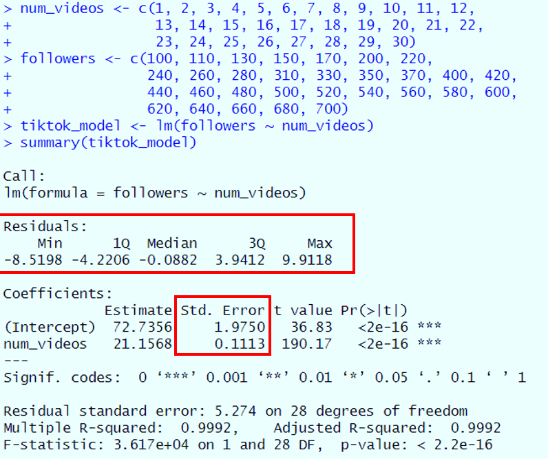
Alright, so you've got your model and your pretty graphs, but hold up! 🛑 We're not done yet. Let's talk about residuals, aka the leftover tea after you've spilled most of it. ☕
Why You Should Care About the Residuals 🤔
Imagine you're trying to predict how many likes your next Instagram post will get. You've got your model, and it's telling you that you'll get around 500 likes. You post it, and boom! You get 505 likes. 🎉 That difference of 5 likes? That's a residual. 🤓
Here's why residuals are super important:
- Accuracy Check 🎯: Residuals help you understand how accurate your model is. If your residuals are all over the place, your model might need a makeover. 💄
- Spotting Outliers 👀: Residuals can help you spot those pesky outliers that could be messing with your model. It's like finding that one friend who always spills the tea but never helps clean up. 🙄
- Improvement Guide 🛠️: By looking at the pattern of residuals, you can figure out how to improve your model. It's like getting constructive feedback on your TikTok dance moves. 💃
- Assumption Check 📜: Remember those assumptions we talked about earlier? Well, residuals can help you check if you're actually meeting them. It's like a reality check for your model. 🤷♀️
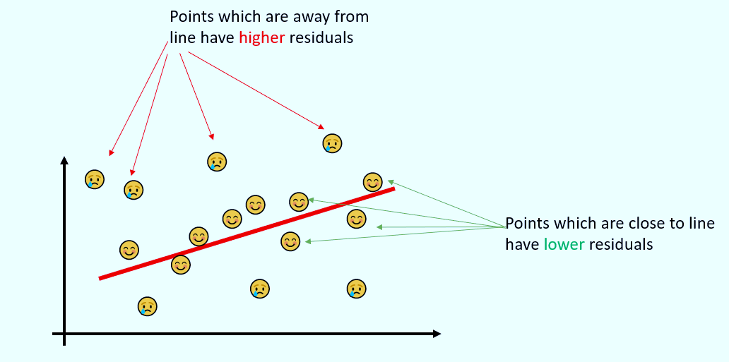
So, are you ready to sip the leftover tea and dive into the world of residuals? 🍵 Let's do it! 🚀
How to interpret the residuals in Simple Linear Regression?
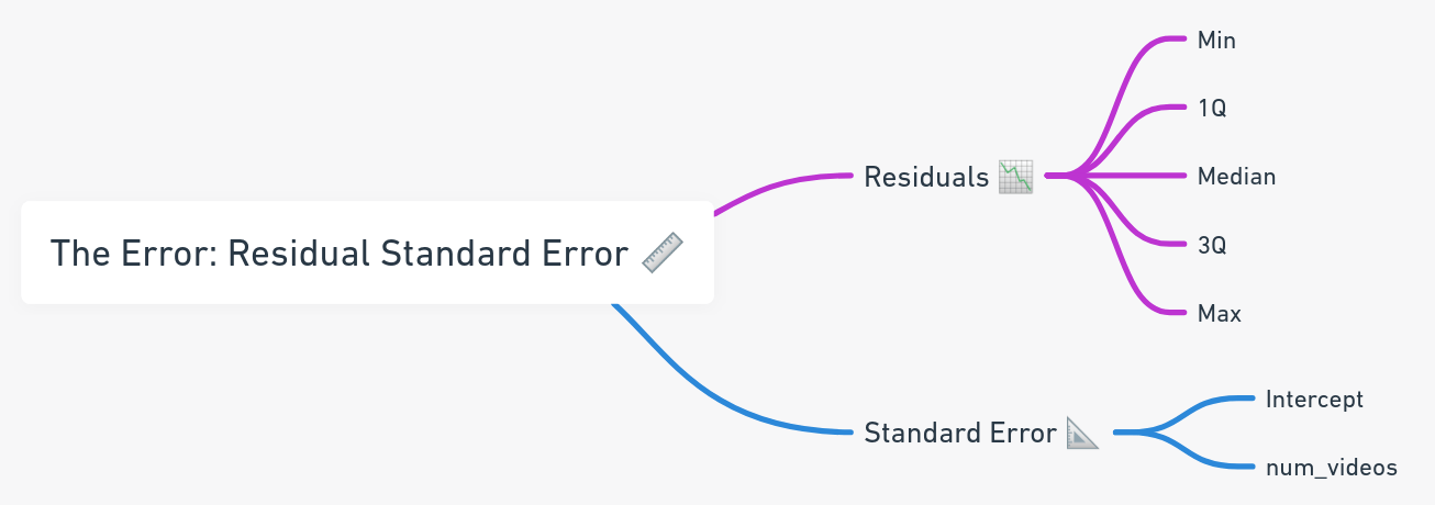
Residuals 📉
- Min (-8.5198): This is the smallest error made by your model. In this case, your model overestimated the number of followers by about 8.5. If your model predicted you'd have 100 followers, you'd actually have around 91.5.
- 1Q (-4.2206): This is the first quartile of your residuals. It means that 25% of the time, your model overestimates your follower count by 4.2 or more. So, if the model says you'll get 200 followers, it could be around 195.8.
- Median (-0.0882): This is the middle value of all the residuals. It's close to zero, which is a good sign! It means that, on average, your model's predictions are pretty spot-on.
- 3Q (3.9412): This is the third quartile. It means that 75% of your residuals are less than or equal to 3.9412. So, 75% of the time, your model will underestimate your follower count by this amount or less.
- Max (9.9118): This is the largest error made by your model. Here, your model underestimated the number of followers by nearly 10. If your model predicted 300 followers, you'd actually have around 309.9.
Standard Error 📐
- Intercept (1.9750): This tells us the average amount that our intercept (72.7356) could "wiggle" due to random chance. A smaller number here is better, as it means our model's starting point is pretty reliable.
- num_videos (0.1113): This is the standard error for the slope of our line, which is 21.1568. Again, a smaller number is better. It means that for each additional video you post, you can expect between 21.0455 and 21.2681 more followers (21.1568 ± 0.1113).
Summary Table 📊
|
Term |
Value |
Detailed Interpretation |
|
Min Residual 📉 |
-8.5198 |
Model overestimated the followers by about 8.5. |
|
Max Residual 📈 |
9.9118 |
Model underestimated the followers by nearly 10. |
|
Intercept Error 📐 |
1.9750 |
Average amount the intercept could vary. Smaller is better. |
|
num_videos Error 📏 |
0.1113 |
Average amount the slope could vary. Smaller is better. |
Assumption Check: Is Your Model Living Its Best Life? 🌟
Normality: Are We Balanced or Skewed? 🍃
Before we get too excited about our model, let's make sure the residuals are normally distributed. This is important because it affects the reliability of the hypothesis tests and predictions.
Code snippet and a histogram or QQ-plot
# Check for Normality
residuals <- tiktok_model$residuals
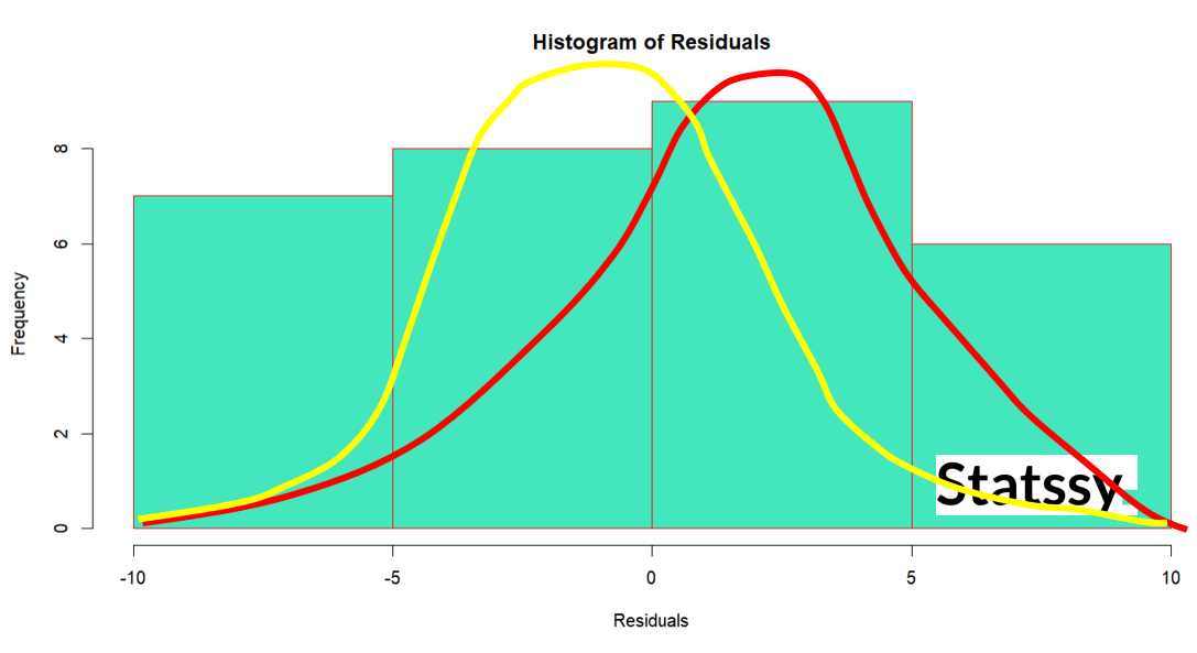
hist(residuals, main = "Histogram of Residuals", xlab = "Residuals", col = "#43e6bd", border = "red")
Here you can see the plot is not a bell shaped perfectly. There is a certain deviation from bell shape.
# QQ-plot
qqnorm(residuals)
qqline(residuals)
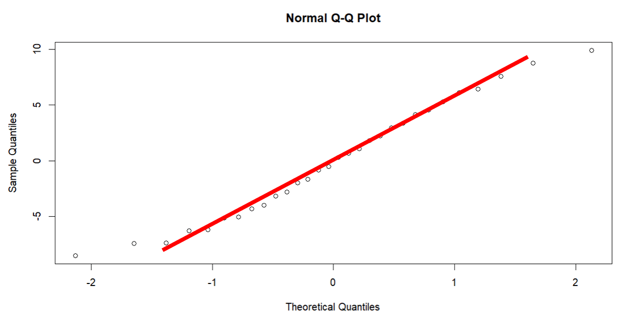
Here you can see the red colored line that I have drawn is not showing that all points follow this line. There is a certain deviation at the end of the line. So we can assume that residuals are linear but not 100% linear.
If the histogram looks like a bell curve or the points in the QQ-plot lie along the line, then the residuals are normally distributed. If not, you might need to consider transforming your data or using a different kind of model.
Heteroskedasticity: Are We Consistent or All Over the Place? 🎭
Heteroskedasticity means that the residuals have non-constant variance across levels of the independent variable. This can mess up the standard errors and thus, your conclusions.
Material: Code snippet and a scatter plot of residuals
plot(tiktok_model$fitted.values, residuals, xlab = "Fitted Values", ylab = "Residuals", main = "Residuals vs Fitted Values")
abline(h = 0, col = "red")
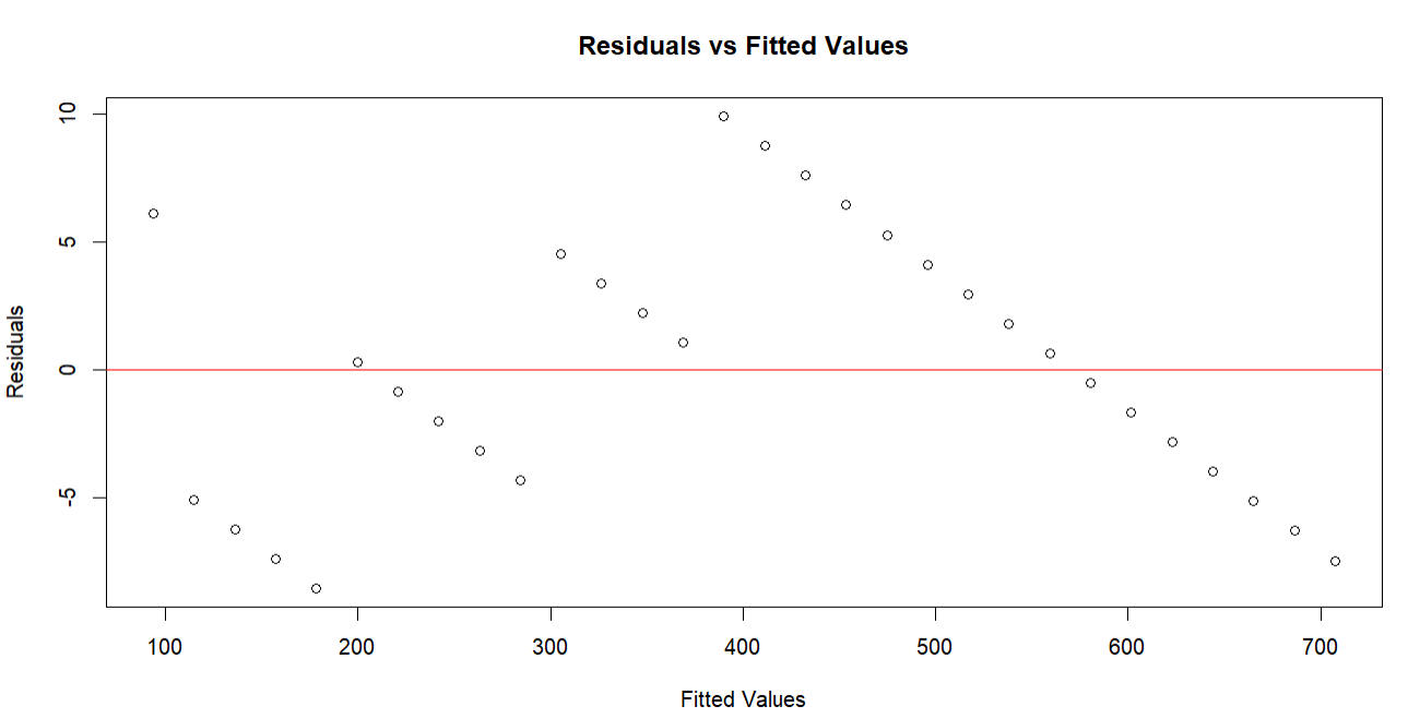
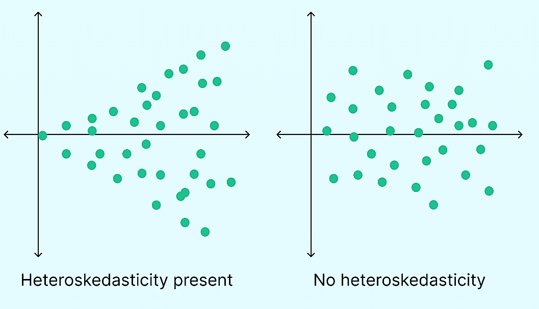
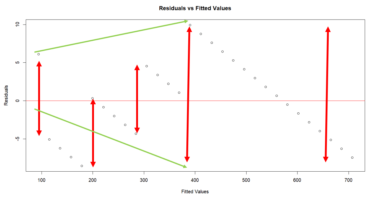
If the plot shows a random pattern (no funnel shape), then the assumption of homoskedasticity holds true. If you see a funnel shape, then heteroskedasticity is present, and you might need to consider transforming your variables or using weighted least squares regression.
For example, check the plots below to understand how constant variance and changing variances look like.
Now let’s see what our plot gives us
Spotting the Drama Queens: Influential Points 🎭
Okay, so you've got your model, your visuals, and you've even sipped the leftover tea with residuals. But wait, there's more! 🛑 Sometimes, your data has what we call "Influential Points," or as I like to call them, the Drama Queens of your dataset. 🎭How to Find and Deal with the Divas in Your Data 👑
Influential points are like the divas in a reality TV show; they demand attention and can totally change the vibe. 🌟 They're data points that have a big impact on your model, and not always in a good way. 😬 Here's why you need to keep an eye out for these drama queens:- Attention Seekers 🌟: These points can skew your model and make it less accurate. It's like that one friend who always steals the spotlight and messes up the group photo. 📸
- Game Changers 🔄: An influential point can change the slope of your line of best fit. Imagine changing the ending of your favorite TV show; that's how big of a deal it is! 📺
- Reality Check 🤔: If you find an influential point, it's a sign you need to check your data. Maybe it's an error, or maybe it's an important piece of information. Either way, you gotta deal with it. 🛠️
# Let's find the drama queens 👑
library(car)  # We'll use the 'car' package for this
influencePlot(tiktok_model)  # This will plot the influential points
)
Now, imagine a plot where most data points are just chilling, but then you have these drama queen points wearing tiny crowns 👑. These are your influential points, and you'll need to decide whether to keep them in the model or kick them out of the party. You will get this plot a list of numbers with some data🎉
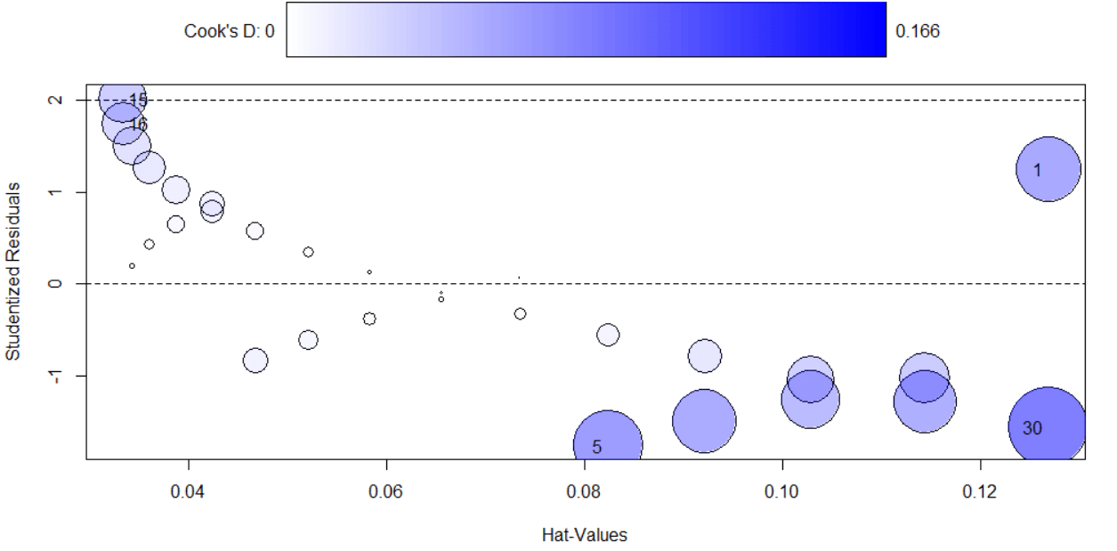

So, are you ready to spot the drama queens in your data and decide if they get to stay in your model's VIP section? 🥂 Let's do this! 🚀
How to find an interpret Influential Points in Simple Linear Regression
StudRes (Studentized Residuals) 🎓
- What it is: These are the residuals that have been standardized. A Studentized Residual greater than 2 or less than -2 is generally considered influential.
- 1.251772: This point is slightly influential but not overly dramatic.
- -1.747046: Again, a bit influential but not a showstopper.
- 2.013021: Ah, a real Drama Queen! This point is highly influential.
- 1.749451: Another influential point, but not as dramatic as the third one.
- -1.546940: Slightly influential but not too dramatic.
Hat 🎩
- What it is: This measures the leverage of each point. Higher values indicate more influence.
- All the values are relatively low, which is a good sign. It means these points aren't overly influential based on their position in the data.
CookD (Cook's Distance) 🍲
- What it is: This is a measure of a data point's influence on the fitted values of a regression model. A value greater than 1 is generally considered highly influential.
- All the values are well below 1, which means none of these points are overly influential based on their impact on the model as a whole.
Summary Table 📊
|
Point |
StudRes |
Hat |
CookD |
Interpretation |
|
1 |
1.251772 |
0.12688172 |
0.11159405 |
Slightly influential but not dramatic. |
|
5 |
-1.747046 |
0.08238784 |
0.12766290 |
A bit influential but not a showstopper. |
|
15 |
2.013021 |
0.03344457 |
0.06321650 |
Highly influential, a real Drama Queen! |
|
16 |
1.749451 |
0.03344457 |
0.04932114 |
Influential but not as dramatic as point 15. |
|
30 |
-1.546940 |
0.12688172 |
0.16563669 |
Slightly influential but not too dramatic. |
So to give you a quick reference

Model Check-Up: Is She Healthy? 🌡️
Alright, you've done a lot so far high five! 🙌 But now comes the moment of truth: Is your model healthy, or does it need some TLC? 🤔 Let's give your model a check-up and see how she's doing. 🌡️
Accuracy Check: No Fake News Here 📏
Last but not least, let's make sure our model is legit. We don't want any fake news here! 🚫
How to Make Sure Your Model Is Legit 🛡️
- RMSE (Root Mean Square Error)
Significance: RMSE is like your model's report card. It tells you how far off your model's predictions are from the actual values. The lower the RMSE, the better your model is at making predictions. 🎯
Formula: The mathematical formula for RMSE is

Here's a code snippet to calculate the RMSE:
# Calculate RMSE 📏
predictions <- predict(tiktok_model)
rmse <- sqrt(mean((followers - predictions)^2))
Imagine a "Verified" badge 💠 popping up next to the RMSE result, just like on a social media profile, to show that your model is legit.
2. MSE (Mean Square Error)
Significance: MSE measures the average squared difference between the observed and predicted values. It's like RMSE but without the square root. 📐
Formula: The formula for MSE is

Here's a code snippet to calculate the MSE:
# Calculate MSE 📐
mse <- mean((followers - predictions)^2)
Imagine a "Verified" badge 💠 popping up next to the RMSE result, just like on a social media profile, to show that your model is legit.
3. MAPE (Mean Absolute Percentage Error)
Significance: MAPE is the drama queen of error metrics. It expresses the forecast errors as a percentage, making it easier to interpret. 🎭
Formula: The formula for MAPE is

Here's a code snippet to calculate the MAPE:
# Calculate MAPE 🎭
mape <- mean(abs((followers - predictions) / followers)) * 100
Imagine a "Verified" badge 💠 popping up next to the RMSE result, just like on a social media profile, to show that your model is legit.
4. MAD (Mean Absolute Deviation)
Significance: MAD measures the dispersion of forecast errors. It's like the chill cousin of MSE and RMSE. 🍹
Formula: The formula for MAD is

# Calculate MAD 🍹
mad <- mean(abs(followers - predictions))

So, are you ready to give your model the check-up she deserves? 🌡️ Let's make sure she's healthy and ready to slay! 🚀
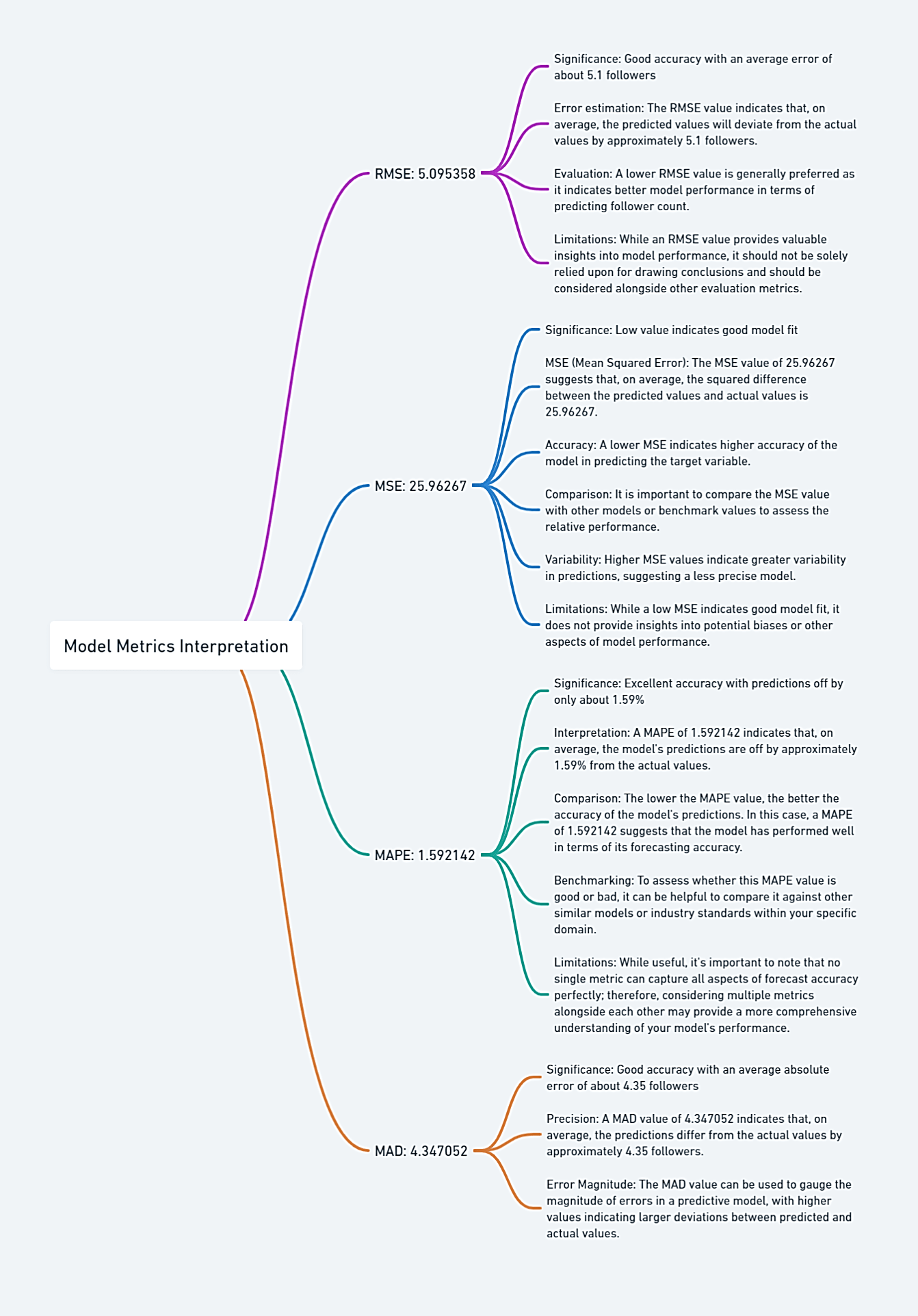
Interpret the accuracy metrics for Simple Linear Regression
Interpretation of RMSE
Value: 5.095358
What it means: RMSE measures the average magnitude of the errors between predicted and observed values. A lower RMSE value indicates a better fit to the data. In our case, an RMSE of approximately 5.1 suggests that our model's predictions are, on average, about 5.1 followers away from the actual number of followers. This is a pretty good result, indicating that our model is quite accurate.
Interpretation of MSE
Value: 25.96267
What it means: MSE is the average of the squares of the errors. It's another way to see how well your model fits the data. A lower MSE is better. Here, an MSE of approximately 26 suggests that the model is doing a good job, as the value is relatively low.
Interpretation of MAPE
Value: 1.592142
What it means: MAPE gives us the average percentage error between the predicted and actual values. A lower MAPE is better, and in our case, a MAPE of approximately 1.59% is excellent. It means our model's predictions are off by only about 1.59% on average, which is quite accurate.
Interpretation of MAD
Value: 4.347052
What it means: MAD measures the average absolute errors. A lower MAD is better. A MAD of approximately 4.35 suggests that the model's predictions are, on average, about 4.35 followers away from the actual values. This is another indicator that our model is doing well.
| Metric | Value | Interpretation |
| RMSE | 5.095358 | Average error is about 5.1 followers. Good accuracy. |
| MSE | 25.96267 | Low value indicates good model fit. |
| MAPE | 1.592142 | Predictions are off by only about 1.59% on average. Excellent accuracy. |
| MAD | 4.347052 | Average absolute error is about 4.35 followers. Another indicator of good accuracy. |
Is Your Model Slaying or Nay? 💅
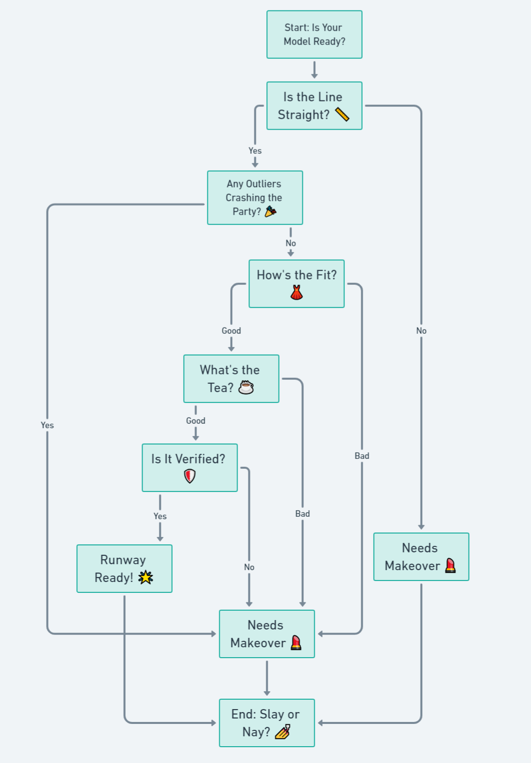
Okay, so you've built your model, checked its health, and even dealt with the drama queens. 🎭 But the ultimate question remains: Is your model runway-ready, or does it need a makeover? 💄 Let's find out! 🌟
How to Tell If Your Model Is Runway-Ready 🎬
Think of this as the final dress rehearsal before your model hits the runway. You want to make sure everything is on point, from the fit to the accessories. 🌟 Here's how to tell if your model is slaying or nay:
- Is the Line Straight? 📏: Look at your scatter plot. Is the line of best fit straight, or is it more like a rollercoaster? A straight line means your model is doing great! 🌈
- Any Outliers Crashing the Party? 🎉: Remember those drama queens? Make sure they're not messing up your model's vibe. 👑
- How's the Fit? 👗: Check the R-squared value. If it's close to 1, your model is fitting like a glove. 🧤
- What's the Tea? ☕: Look at the residuals. Are they close to zero? If yes, then your model is spill-proof! 🍵
- Is It Verified? 🛡️: Finally, check the RMSE value. A low RMSE is like getting the verified badge on social media. 💠
If your model passes all these checkpoints, then girl, she's ready to slay that runway! 🚀 But if not, no worries—every model needs a little touch-up now and then. 💄
# Finding the total drama 🎭
sst <- sum((followers - mean(followers))^2)
When you run the code you will get this

Interpretation of Sum of Squares Total (SST) 🎭
Value of SSR
- SST: 1006787
What it means
- Sum of Squares Total (SST)is a measure of the total variability within your data. In simpler terms, it's like the total "drama" or "buzz" around your TikTok followers. It tells you how much the number of followers varies around the mean number of followers.
- In our case, the SST value is 1006787. This is a pretty large number, indicating that there's a significant amount of variability in the number of followers. This could be due to various factors like the type of content you post, the time you post, or even random fluctuations in follower count.
Why it's important
- Knowing the total variability is the first step in understanding how well your model will be able to predict the outcome. If SST is high, it means there's a lot to explain, and a good model will be able to account for a large portion of this variability.
The Trendsetter: Sum of Squares Regression 📈
Next, let's talk about the Sum of Squares Regression. This is the part of the variability that your model actually explains. It's like the trending topics that everyone is talking about. 🗣️
What It Is and How to Find It 📊
- Sum of Squares Regression (SSR): This is the variability that your model explains. It's like the trending hashtags that everyone is using. 📈

# Finding the trendsetter 📈
ssr <- sum((predict(tiktok_model) - mean(followers))^2)
When you run this code, you will get this

Interpretation of Sum of Squares Regression (SSR) 📈
Value of SSR
- SSR: 1006008
What it means
- Sum of Squares Regression (SSR)measures how much of the total variability (or drama) in your TikTok followers is explained by your model. Think of it as the "trendsetting" power of your model. The higher this number, the better your model is at capturing the trends in your data.
- In our case, the SSR value is 1006008, which is very close to the SST (Total Sum of Squares) of 1006787. This suggests that our model does an excellent job of capturing the variability in the number of followers.
Why it's important
- A high SSR value relative to SST means that your model is effective in explaining the variability in the data. This is a good sign that your model is robust and reliable for making predictions.
The Oopsies: Sum of Squares Error 😬
Last but not least, let's talk about the Sum of Squares Error. This is the variability that your model doesn't explain. It's like the bloopers and mistakes that didn't make the final cut. 🎬 What It Is and How to Find It 🤔- Sum of Squares Error (SSE): This is the variability that your model doesn't explain. It's like the deleted scenes and bloopers from a movie. 😬
# Finding the oopsies 😬
sse <- sum((followers - predict(tiktok_model))^2)
When you run this code, you will get this

Interpretation of Sum of Squares Error (SSE) 😬
Value of SSE
- SSE: 778.8802
What it means
- Sum of Squares Error (SSE)measures the amount of variability in your TikTok followers that your model couldn't explain. Think of it as the "oopsies" or the "misses" of your model. The lower this number, the better your model is at fitting the data.
- In our case, the SSE value is 778.8802, which is much lower compared to the SST (Total Sum of Squares) of 1006787 and the SSR (Sum of Squares Regression) of 1006008. This suggests that our model does an excellent job of fitting the data, leaving only a small amount unexplained.
Why it's important
- A low SSE value means that the errors between the predicted and actual values are small, indicating a good fit. This is a good sign that your model is reliable for making predictions.
So lets summarize everything we found.
|
Metric |
Value |
Interpretation |
|
SST |
1006787 |
High variability in the number of followers. A good model should be able to explain this variance. |
|
SSR |
1006008 |
High SSR indicates the model effectively captures the variability in the number of followers. |
|
SSE |
778.8802 |
Low SSE indicates the model effectively fits the data, leaving only a small amount unexplained. |

# New data: Let's say you're planning to post 10 more videos 📹
new_data <- data.frame(num_videos = c(31:40))

# Ask the crystal ball 🔮
future_followers <- predict(tiktok_model, newdata = new_data)

Now we can also show these predictions on the chart.

# Existing data
existing_data <- data.frame(num_videos = num_videos, followers = followers)
# Future predictions
future_followers <- predict(tiktok_model, newdata = new_data)
# Future data
future_data <- data.frame(num_videos = c(31:40), followers = future_followers)
# Combine existing and future data
all_data <- rbind(existing_data, future_data)

# Create the ggplot
ggplot(all_data, aes(x = num_videos, y = followers)) +
  geom_point(aes(color = ifelse(num_videos <= 30, "#43e6bd", "red")), size = 4) +  # Color points based on existing or future data
  geom_smooth(data = subset(all_data, num_videos <= 30), method = "lm", se = FALSE, aes(color = "#43e6bd")) +  # Line of best fit only for existing data
  scale_color_identity(name = "TikTok Followers",
                       labels = c("Existing Data", "Predicted Followers"),
                       breaks = c("#43e6bd", "red"),
                       guide = "legend") +
  labs(title = "Predicting Future TikTok Followers",
       x = "Number of Videos",
       y = "Number of Followers") +
  theme_minimal()  # Keep it clean
It's like a magical moment where the numbers roll out, and voila! You've got your future follower count. 🌟
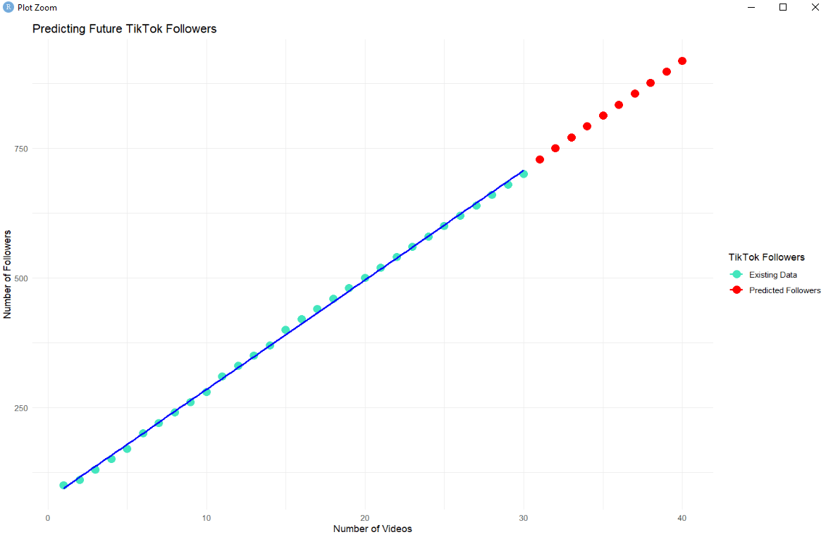
Let’s see what we did here,
|
Step No. |
Description |
Code Segment or Function Used |
|
1 |
Create new data for predicting future followers for videos 31 to 40 |
new_data <- data.frame(num_videos = c(31:40)) |
|
2 |
Use the existing model to predict future followers |
future_followers <- predict(tiktok_model, newdata = new_data) |
|
3 |
Create a data frame for existing data |
existing_data <- data.frame(num_videos = num_videos, followers = followers) |
|
4 |
Create a data frame for future predicted data |
future_data <- data.frame(num_videos = c(31:40), followers = future_followers) |
|
5 |
Combine existing and future data into one data frame |
all_data <- rbind(existing_data, future_data) |
|
6 |
Create a ggplot to visualize both existing and future data |
ggplot(all_data, aes(x = num_videos, y = followers)) |
|
7 |
Add points to the plot, color-coded based on whether they are existing or future data |
geom_point(aes(color = ifelse(num_videos <= 30, "#43e6bd", "red")), size = 4) |
|
8 |
Add a line of best fit based on existing data |
geom_smooth(data = subset(all_data, num_videos <= 30), method = "lm", se = FALSE, aes(color = "#43e6bd")) |
|
9 |
Customize the color legend and labels |
scale_color_identity() and labs() |
|
10 |
Apply a minimal theme to the plot |
theme_minimal() |
So, are you ready to play the prediction game and see what your data crystal ball has to say? 🤩 Let's do it and make some data magic happen! 🌟🔮
The Quality Check: Is Your Model A-List or D-List? 🌟
Alright, you've done the work, you've made your predictions, but now comes the ultimate question: Is your model A-List or D-List? 🤩🤔 We're talking red-carpet ready or not even fit for the discount bin. 🌟🗑️
A Final Checklist to Make Sure Your Model is Red-Carpet Ready 📋
- Adjusted ( R^2 ) Score: Is it close to 1? If yes, your model is a superstar! 🌟
- F-Statistic: Is it significantly high? Then your model is the judge's favorite! ⚖️
- Residuals: Are they randomly scattered? If so, your model is keeping it real! 🎯
- Outliers: Any drama queens? If not, your model is drama-free! 🎭
- Coefficients: Are they significant? Then your model has star power! 🌠
- RMSE (Root Mean Square Error): Is it low? Then your model is accurate! 🎯
Material: Picture an interactive checklist where each item has a checkbox next to it. When you check off an item, a fun emoji pops up:
- Adjusted ( R^2 ) Score: 🌟
- F-Statistic: ⚖️
- Residuals: 🎯
- Outliers: 🎭
- Coefficients: 🌠
- RMSE: 🎯
- MAPE 🎯
So, is your model ready for the big leagues? 🏆 Is it ready to strut its stuff on the data runway? 🐾 Use this checklist to make sure your model is not just good, but red-carpet ready! 🌟
Wrapping It Up: You Did It! 🎉
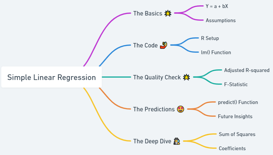
OMG, you made it! 🎉 You've gone from a data newbie to a budding data diva, and I couldn't be prouder! 🌟 You've learned the ABCs of Simple Linear Regression, you've crunched the numbers, and you've even peeked into the future with your very own data crystal ball. 🔮
A Recap of This Fab Journey 🌈
- The Basics: You learned what Simple Linear Regression is and why it's the ultimate tool for both data newbies and pros. 🌟
- The Code: You got your hands dirty with R code, and you even predicted your future TikTok followers! 🤳
- The Quality Check: You made sure your model is A-List and red-carpet ready! 🌟
- The Predictions: You used your model to make future predictions. How cool is that? 🤩
- The Deep Dive: You went into the nitty-gritty details to understand your model better. 🕵️♀️
What's Next? 🌠
So what's next on this fabulous data journey? Well, the sky's the limit! 🌌 You can dive into multiple linear regression, explore different types of data visualization, or even start your own data project. 🚀
You've got the tools, you've got the talent, and now you've got the confidence to take on the data world. 🌍 So go out there and make some data magic happen! 🌟✨
And remember, this is just the beginning. The world of data is vast and exciting, and you're now officially a part of it. 🌍🌟
So go ahead, take a bow, you've earned it! 🙇♀️🎉

